 Enrichyouenergy
How CMU's Intro Programming Course Teaches Efficiency

From timing a program to reasoning about how its work grows, efficient programming is not only about finding a solution, but also about figuring out the heuristics
A loop can run over a million-element list and still do only four iterations. Another loop can contain i**2 and take square-root time.
Both examples made me pause while studying efficiency. I could read the Python. What I was learning was how to read the amount of work behind it.
These notes grew out of the efficiency material in CMU’s 15-112, Fundamentals of Programming and Computer Science. CMU lists both efficiency and algorithm analysis among the topics of this introductory Python course. Its Unit 8 brings efficiency together with sets and dictionaries.
The question connecting everything is simple:
When the input gets bigger, how much more work does the program do?
Start with a problem worth making faster
Suppose we want the largest sum of two elements at different positions in a list containing at least two numbers.
One approach checks every pair. Another finds the two largest values in a single pass, allowing equal values when they occur at different positions, and adds them.
The first examines N(N − 1)/2 pairs. The second visits N elements while maintaining two values.
If the list grows from 100 elements to 10,000, the number of pairs grows from 4,950 to 49,995,000. A single scan grows from 100 visits to 10,000.
Both approaches can produce the same answer. Their workloads grow very differently.
That gives efficiency a purpose before we introduce any notation. It helps us choose an approach that remains usable as the problem grows.
Timing is useful. It answers a particular question.
The notes introduce elapsed-time measurements using time.time(). This makes the difference between algorithms visible, but the readings vary across runs and machines.
For a short duration measurement, Python provides time.perf_counter(). For repeated measurements of small snippets, it provides timeit.
from time import perf_counter

start = perf_counter()
result = algorithm(data)
elapsed = perf_counter() - start
A measurement tells us how long a particular execution took under particular conditions. It does not, by itself, establish how the algorithm scales.
I would therefore be careful with the conclusion “we cannot compare programs using time.” Practical performance work depends on it, but we also need a way to reason beyond one experiment.
That is where counting work becomes useful.
Define N, then count work
For a list, we usually define N as its length. We then count operations under a stated cost model.
In the examples here, indexing and arithmetic on ordinary, bounded-size numbers are treated as constant-time operations. That assumption lets us focus on the algorithm’s structure.
A linear search illustrates the idea. To determine whether a value is in an unsorted list, we inspect elements until we find it or reach the end.
The best case finds it immediately. The worst case inspects all N elements. The course notes I studied emphasize worst-case analysis, so that is the starting point here.
One detail matters: Big O does not itself mean worst case. We can use Big O to describe a worst-case, average-case, or best-case running-time function. We must say which one we mean.
Big O describes growth
Imagine a step count of:
4N² + 17N + 20As N grows, the quadratic term dominates. In introductory analysis, we discard the lower-order terms and constant coefficient and describe the growth as O(N²).
More precisely, Big O is an asymptotic upper bound. Θ(N²), read “Theta of N squared,” expresses a tight bound when the function really grows at that rate. The course’s function-family shorthand is a useful entry point; keeping this distinction in mind prevents confusion later.
The common growth rates are:
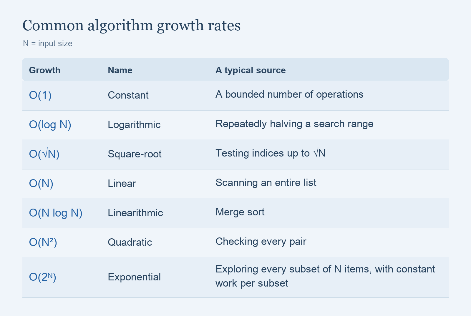
These are growth patterns, not stopwatch readings. Constants, input structure, and implementation details still matter in practice, especially for small inputs.
Searching: preparation changes the total cost
Linear search takes O(N) worst-case time. Binary search uses a sorted list and repeatedly discards half the remaining range, taking O(log N) time with constant-time indexing and comparisons.
The logarithm becomes intuitive when we ask how many halvings it takes to reduce the candidate range to about one element. A range of roughly a million elements takes about twenty halvings.
But binary search needs sorted data. If the list starts unsorted, we must include the preparation cost.
For Q searches:
Repeated linear search: O(QN)
Merge sort once, then binary search: O(N log N + Q log N)
When Q = N, these become O(N²) and O(N log N). Sorting once is asymptotically more efficient.
When Q = 1, a single O(N) scan is asymptotically cheaper than first sorting the list in O(N log N).
This was a useful shift in perspective for me. “Which search is faster?” becomes a more complete question when we include how often we will search and what preparation is required.
Also, sorting a Python list does not make x in values use binary search. List membership still scans; binary search requires a suitable implementation, such as one built around bisect.
Sorting: understand where N log N comes from
Selection sort repeatedly scans the remaining unsorted elements to choose the next value. The number of comparisons is:
(N − 1) + (N − 2) + ... + 1 = N(N − 1) / 2That gives O(N²).
Merge sort combines already sorted groups into larger sorted groups. Across a whole level, it processes O(N) elements. Group sizes double at each level, creating O(log N) levels.
Multiply those two quantities:
O(N) work per level × O(log N) levels = O(N log N)The course’s approximate 3N log N count belongs to its simplified model of comparisons and copying. The coefficient is not a universal count for every implementation.
Python’s built-in sorting is adaptive and merge-based, commonly described as Timsort; current CPython uses the Powersort merge strategy. It can exploit existing order. The important point for this article is to account for sorting as O(N log N) in the worst case when comparisons take constant time.
Takeaways
My most useful takeaway is a habit of asking a few questions before calculating:
- What is the input size?
- How many times does each operation run?
- How much work is hidden inside each operation?
- Have I included preparation and memory costs?
- Am I describing worst-case or the average-case?
Then I can measure the program and see whether the reasoning explains what happens.
Python gives these questions concrete examples, but they travel well to other languages, such as C, which I am going to learn next semester. The syntax and library costs may change. The habit of tracing work as the input grows remains useful.
For me, that is what makes efficiency worth learning early: I can look at a correct program and begin to explain how it will behave on a larger problem. This is why I chose to write this article and share it with more people.
This article is based on my study notes and the supplied CMU 15-112 Unit 8 summary. Examples and reflections are my own presentation of the ideas; this article is not affiliated with or endorsed by CMU.